
Speaker Embeddings Explained: From i-Vectors to ECAPA-TDNN and WavLM
Understand how speech becomes a speaker vector, how i-vectors, x-vectors, ECAPA, residual networks and WavLM differ, and why compatible checkpoints, aggregation and evaluation matter more than a vector label.
Sources checked · Cyber Search MatchA speaker embedding is a learned or statistically estimated representation of a speech passage, not a permanent fingerprint that removes every recording effect. Different methods produce different spaces and require compatible preprocessing and scoring. Compare independent recordings under a declared protocol, and distinguish a model family from its trained checkpoint, runtime and application. CS Match primarily uses normalized ECAPA vectors with cosine scoring.
A vector represents an observation, not an immutable person
The input to an encoder is recorded speech from a particular interval. Its vector therefore reflects both information useful for comparing speakers and the conditions under which that speech was captured. Wording, channel, background sound and available duration can affect the representation. Calling it a voiceprint does not remove those dependencies or turn each coordinate into a directly interpretable physical measurement.
The objective is to make relevant observations from one speaker sufficiently consistent while separating different speakers under the intended conditions. That is an empirical learning and evaluation problem. A model can produce stable vectors on its familiar training distribution and behave differently on short telephone speech, a distant microphone or an unfamiliar language.
Use a representation as one component of a defined comparison task. Pairwise verification, search across enrolled references and clustering a conversation impose different decision policies. A close pair of vectors is not automatically a verified name, a transcript or a result that the speaker was physically present when the original recording was made.
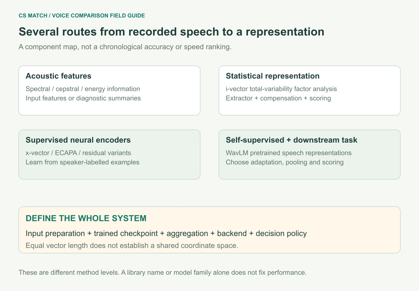
Acoustic features and speaker embeddings occupy different levels
A waveform can first be expressed as short-time spectral or cepstral features. MFCCs summarize aspects of the spectral envelope over successive frames; librosa documents the coefficient sequence and its configurable extraction. Such features can feed a learned model or a statistical extractor. A raw MFCC frame is not the same thing as an utterance-level neural speaker embedding.
Aggregation matters. Averaging acoustic coefficients, estimating a statistical latent representation and running an encoder trained to distinguish speakers are different operations. They may all return arrays of numbers, but their coordinates and score distributions are not interchangeable. A shorter summary can be useful for signal diagnostics without demonstrating the discrimination expected from a dedicated speaker model.
This distinction is relevant to our fallback paths. The code can construct librosa acoustic summaries or RMS-based features when the main model is unavailable. Those representations describe aspects of the sound through a different mechanism. A report should retain which engine produced the output, and an evaluation should not mix its scores with ECAPA results as though only processing speed changed.
i-Vectors model total variability through factor analysis
The i-vector approach compresses recording statistics into a low-dimensional latent representation. Dehak and colleagues describe a total-variability space that contains speaker and channel variation together. Its estimation uses statistics relative to a background model, rather than directly applying the supervised neural speaker classifier familiar from many newer systems.
Channel compensation and scoring are consequently important parts of the method. The original work examines transformations intended to reduce nuisance variation before comparison. An i-vector does not promise that a microphone or session effect has disappeared simply because the result is compact. The complete extractor and scoring arrangement defines the actual verification system.
Treat this architecture as an informative baseline and historical foundation. Its usefulness depends on training resources, target conditions and the evaluation protocol, not its age alone. When comparing it with a neural alternative, keep the input and trials consistent. A recognizer tested on easier or longer recordings cannot be declared better solely by placing its reported percentage beside a result from another experiment.
x-Vectors learn to distinguish training speakers
The x-vector approach trains a neural network to discriminate training-speaker classes and extracts a fixed-dimensional utterance representation for subsequent comparison. Frame-level processing and temporal statistics pooling accommodate variable-duration speech. The resulting embedding can be used for speakers outside those training classes; the training classifier's label list is not the application's identity database.
Snyder and colleagues study noise and reverberation augmentation in this supervised framework and compare with i-vector baselines under stated conditions. That provides evidence about a particular architecture and experimental setup. It does not mean every implementation called x-vector has identical weights, augmentation, robustness or performance on arbitrary uploaded recordings.
Separate network training from the backend used to compare extracted vectors. A pipeline may transform vectors, use cosine scoring or fit another scoring model. Keep these choices in the comparison record. Replacing the encoder while retaining old score thresholds can change which recordings are accepted even when the surrounding report still displays the same metric names.
ECAPA-TDNN refines temporal features and pooling
ECAPA-TDNN develops the TDNN speaker-embedding approach with multi-scale temporal processing, channel attention and feature aggregation. Its paper describes Res2Net-style modules, squeeze-and-excitation mechanisms and channel-dependent attentive statistics pooling. These choices aim to use informative temporal and channel structure when summarizing an utterance, rather than treating every frame contribution identically.
The architecture specifies how a representation is computed; trained weights specify what was learned from a particular dataset and objective. Our configured SpeechBrain checkpoint is one concrete ECAPA implementation. It should be identified by its model package and preprocessing rather than presented as interchangeable with every model carrying the same architecture name.
Attention is a learned weighting mechanism, not a guarantee that the system has isolated the intended speaker. Background speech, overlapping participants or a reference assembled from several voices can still affect the result. Inspect the selected interval and test target conditions independently before converting architectural sophistication into a claim about a completed real-world task.
Residual encoders offer another representation family
Residual networks provide a different way to build deep feature extractors, using skip connections while processing acoustic inputs. Deep Speaker is an early end-to-end neural embedding example that discusses convolutional and recurrent alternatives and learned speaker comparison. A residual backbone is a design choice, not a single standard checkpoint with a universal voice-comparison score scale.
The input representation, pooling and training objective remain consequential. Two residual speaker encoders can differ in spectral features, depth, augmentation and output dimension. Comparing only the backbone name hides these changes. Keep the entire model package and backend attached to any measured result, including the source duration and acquisition conditions used in evaluation.
An application should choose among encoders through matched trials and its resource budget. A larger network may or may not improve the specific failure that matters, and its inference cost depends on implementation and hardware. Preserve a baseline so a proposed replacement can be assessed through gained and lost comparisons rather than through the appeal of a newer family name.
WavLM separates broad pretraining from a speaker task
WavLM learns general speech representations through self-supervised pretraining, combining masked prediction with denoising-related training. Its paper addresses several downstream speech tasks, including speaker-related applications. A general pretrained representation is therefore a starting point for a task-specific system, not automatically a drop-in replacement for a complete speaker encoder and scoring policy.
Speaker verification requires choices about extracted layers, aggregation, downstream training and comparison. The official implementation distinguishes model sizes and downstream configurations. These choices can change quality and resource use. A result from one WavLM-based verification system should not be assigned to every use of a WavLM feature extractor or to an unrelated transcription workflow.
For our recorded-review task, a WavLM-based candidate would need compatible preprocessing, independent target trials and deployment measurements before replacement. Evaluate short passages, channel mismatch and multilingual conditions rather than relying only on a broad benchmark headline. The current CS Match code path described here remains ECAPA-based; this section introduces an alternative research family, not a newly installed model.
Training objectives shape which differences matter
Supervised speaker classification, margin-based objectives and metric-learning losses encourage different relationships among training examples. The class identities used during training provide supervision; deployment can still compare unseen speakers through the resulting representation. A useful objective needs suitable data, sampling and evaluation, rather than a label suggesting it directly solves every downstream decision.
Generalized end-to-end loss is one published example of training around speaker-embedding comparisons and difficult examples. It illustrates that the learning objective is a distinct component from a backbone or inference library. Its reported experimental improvements belong to that paper's system and conditions; they are not evidence that our current worker uses that loss or reproduces its results.
Training data also determines which variation the system encounters. Multiple sessions per speaker and appropriate augmentation can expose channel changes, while data leakage can inflate evaluation. Record the checkpoint's dataset and protocol before reusing an error rate. A small set of self-comparisons cannot reveal how well an objective distinguishes new speakers across independent recordings.
Compatible vectors require more than matching dimensions
A coordinate is meaningful only within its model's representation space. Two encoders can emit vectors of the same dimension while assigning entirely different meanings to corresponding positions. Directly comparing them element by element does not become valid because the arrays have equal length, and truncating unequal arrays is not a learned transformation between their spaces.
Keep reference and query generation tied to the same compatible model, preprocessing and normalization. After a checkpoint change, regenerate stored references or use an explicitly trained and evaluated compatibility method. Also record the sampling rate and input convention. A decoder accepting the file format does not establish that the encoder received the representation it was trained to use.
The practical diagnostic is provenance: which engine and version generated each vector? Our helper functions do not establish learned compatibility between ECAPA, librosa and RMS representations. Mixed-engine results therefore require separate treatment and validation. This is a current evaluation boundary, not a claim that cross-model alignment or score calibration has already been implemented.
| Item to keep compatible | Why it matters | Insufficient shortcut |
|---|---|---|
| Encoder and checkpoint | Defines the coordinate space | Equal vector length |
| Signal preparation | Defines the input seen by the encoder | Same filename extension |
| Aggregation and scoring | Defines the comparison rule | Same similarity label |
| Engine provenance | Exposes fallback or version changes | A completed task alone |
Cosine and PLDA answer through different scoring models
Cosine similarity measures the normalized dot product of two nonzero vectors. Multiplying one vector by a positive scalar leaves this direction-based score unchanged. That mathematical property does not remove noise or channel effects from the representation. It also does not make the result a posterior probability that two recordings contain the same speaker.
PLDA uses a fitted probabilistic model of speaker-related variation. Kaldi's documented backend includes a transformation based on within- and between-class variation and a same-versus-different log-likelihood ratio. Such a score is not numerically interchangeable with cosine. Its training population, transforms and calibration affect how a downstream application should use it.
For comparison, fix the encoder and evaluate candidate backends on the same independent trials before changing both at once. A threshold belongs to a defined score distribution and task. CS Match currently uses cosine to its reference centroid; it does not implement the PLDA backend described here or convert that cosine into a calibrated identity probability.
Cosine(x,y) = (x · y) / (||x|| ||y||), for nonzero vectors in a compatible space.A centroid can summarize or dilute a reference
Averaging window embeddings is a simple reference aggregation rule. It combines several observations and can reduce sensitivity to one unusual window, but it can also mix distinct voices or recording conditions. Inspect the contributing speech and preserve the aggregation policy. A larger profile is not automatically a better representation of the intended speaker.
In a deliberately invented two-dimensional example, reference vectors A=(1,0) and B=(0,1) have mean (0.5,0.5). Normalizing gives approximately (0.707,0.707), whose cosine with A is approximately 0.707. A reference containing A alone would have cosine 1 with A. These axes are arithmetic coordinates, not measured voice features, actual speakers or a projection of learned embeddings.
The example shows how a mixed profile changes the comparison direction without proving how much any real recording will be affected. Our profile uses normalized averaging and records supporting window information. Check that sample's content and compare independent passages before interpreting consistency diagnostics or a strongest individual-window score as evidence that the reference itself is well formed.
Invented unit vectors: A=(1,0), B=(0,1); normalized mean=(1/√2,1/√2).Cosine(A, normalized mean)=1/√2≈0.707; cosine(A,A)=1. Not a voice accuracy result.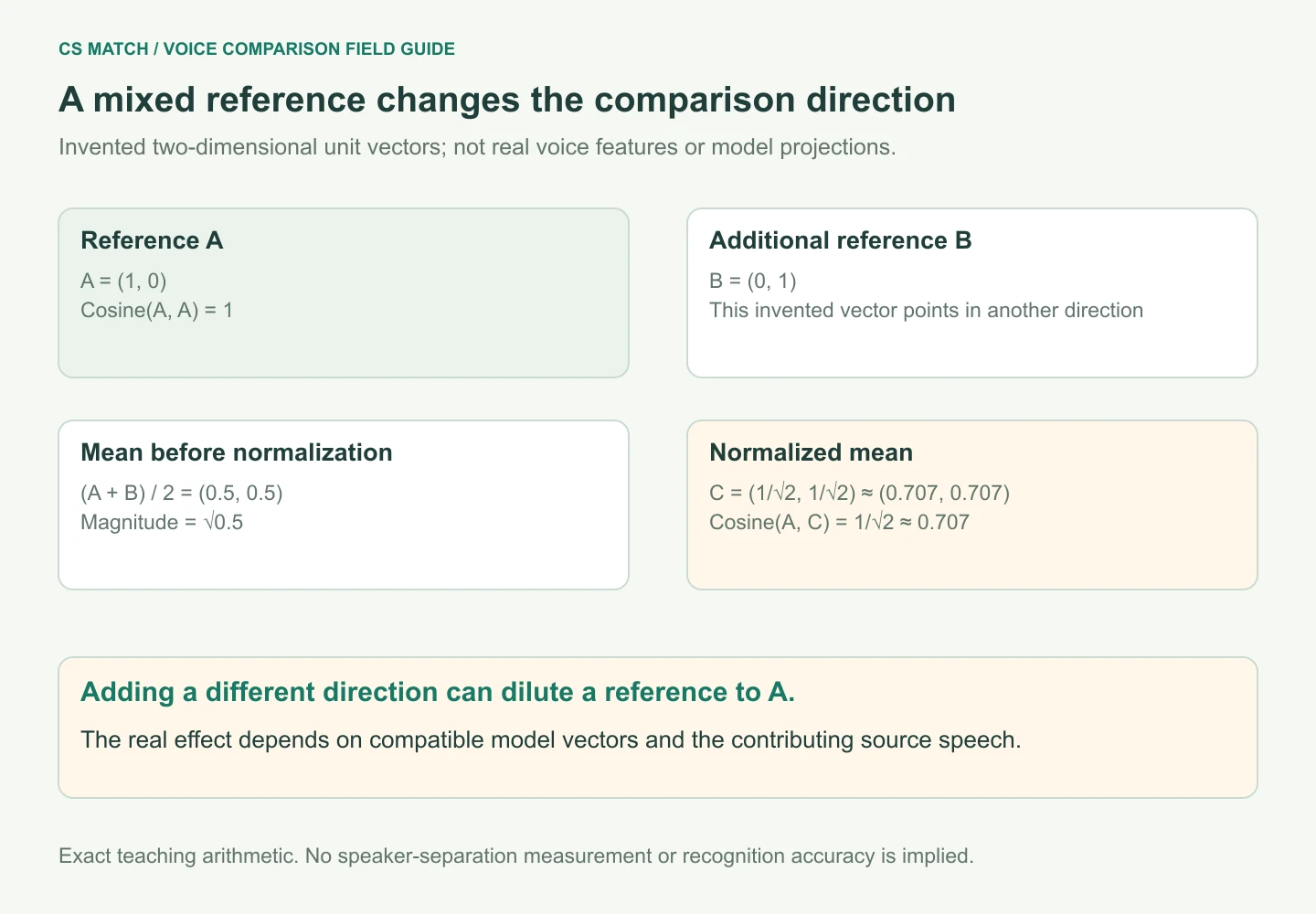
Choose an encoder through independent task evidence
Compare complete systems on declared same-speaker and different-speaker trials, including independent sessions, relevant channels, languages and source durations. NIST's evaluation protocol explicitly describes enrollment and test conditions. Its structure is a useful example of defining the task before reporting results, rather than treating one embedding family as inherently best for every recording.
Record the encoder, checkpoint, preparation, aggregation, scoring backend and threshold together. Separate a component benchmark from the long-recording search that selects its best windows. Several favourable opportunities in one recording can change the distribution of maximum scores. Include failed or degraded-mode tasks instead of evaluating only examples where the preferred model happened to run successfully.
For the current product, normalized ECAPA embeddings and inspectable source windows form a practical modular baseline. The justified next change is one that improves relevant paired comparisons while meeting the processing budget. This article explains the available representation families; it does not publish a new CS Match error rate, introduce another encoder or establish automatic identity verification.
Questions about this workflow
Is an embedding a unique permanent identifier for a voice?
No. It represents recorded speech under a particular model and processing setup. Conditions and duration can change it, and similarity needs independent evaluation for the intended task.
Can equal-length vectors from different models be compared directly?
Equal length does not establish a shared coordinate space. Use compatible generation or an explicitly learned and validated mapping, and retain engine/version provenance.
Is WavLM automatically better than ECAPA for our recordings?
No conclusion follows from the family name alone. Compare suitable checkpoints, downstream configurations, source conditions and runtime on the same independent trials.
Why can a mixed reference reduce similarity to a clear passage?
Averaging different representations changes the profile direction. The invented two-dimensional example demonstrates the arithmetic; the actual effect must be measured on supported recordings.
Continue with the next useful step
How Voice Comparison Works: From Recording to Reference Match
Follow the complete voice-comparison pipeline: source preparation, speech detection, windows, speaker embeddings, reference profiles, similarity scoring and source-linked review, with the current CS Match implementation explained.
What Voice Similarity Scores Mean
Understand best score, top 5 median, matched speech, speaker summaries and technical similarity labels without treating them as identity probabilities.
How to Read an Audio Analysis Report
Understand source players, quality indicators, transcripts, speaker groups, voice similarity and signal charts in the current Audio Analysis report.