
Speaker Verification Metrics: FAR, FRR, EER, minDCF and Calibration
Read voice-verification metrics correctly: trial labels, false accepts and rejects, ROC and DET, EER, detection costs, calibration, uncertainty and the limits of current report scores.
Sources checked · Cyber Search MatchSpeaker-verification metrics describe performance on labelled trials under a declared decision rule. FAR and FRR measure different conditional errors; EER summarizes a balanced-error point; detection cost adds explicit priorities; calibration gives scores a decision-related meaning. None turns a raw cosine percentage into a probability of identity. Evaluate the actual workflow, report its denominators and preserve independent evidence for the chosen threshold.
Define the trial and the positive class first
A verification trial contains a reference or enrollment side, a test side and a known relationship. A target trial contains the intended speaker under the declared task; a non-target trial does not. For a mixed test recording, define whether presence anywhere, presence in a selected passage or another condition constitutes a target. The same audio can support different questions with different labels.
State the decision unit alongside that relationship. A score for one window, a score for a pair of clean excerpts and the maximum over a long recording are not interchangeable observations. Each can be evaluated, but its denominator and selection rule must remain fixed. A count of windows should not be advertised as a count of independent people or calls.
For the examples below, higher scores favour the target hypothesis and accepting means that the score meets the chosen threshold. This convention makes false accepts and false rejects unambiguous. It does not assert that a technical acceptance establishes personal identity. Our current tool supports review of supplied sources, not a complete verified-enrollment or authentication process.
Separate similarity, ranking and probability
A cosine score describes the relationship between compatible vectors. A display can rescale it or organize it into categories without learning a probability model. A number shown as a percentage therefore needs its definition. It might describe similarity or coverage, rather than the chance that two recordings contain the same person under a specified population and prior.
Ranking asks whether target trials generally score above non-target trials. Calibration asks whether numerical scores support decisions with their intended interpretation. A strictly increasing remapping preserves ordering and the attainable threshold tradeoffs, yet changes which numerical cutoff corresponds to a decision. Good ranking is valuable, but it does not by itself supply a meaningful probability scale.
Keep this distinction when comparing interfaces. Two products can display different percentages for the same underlying ordering, while identical-looking percentages can have unrelated definitions. Read the model, scoring rule, aggregation and decision policy before comparing numbers. In CS Match, cosine to the normalized reference centroid and its configured categories remain technical measures rather than calibrated identity probabilities.
FAR and FRR use different denominators
False acceptance rate is the fraction of non-target trials accepted at the specified threshold. False rejection rate is the fraction of target trials rejected. In detection terminology these correspond to false-alarm and miss probabilities. State the positive class, inequality and treatment of ties; labels such as false positive are otherwise easy to reverse when a task is described informally.
Consider invented counts: one hundred target trials and one thousand non-target trials. A stricter threshold rejects ten targets and accepts two non-targets. Its FRR is ten percent and its FAR is 0.2 percent. The denominators differ because the questions differ. Dividing both error counts by all eleven hundred trials would produce another statistic and conceal the conditional rates.
These are teaching counts, not a CS Match test set or a recommended operating point. Their overall target proportion also need not equal a deployment prior. Preserve the counts beside the percentages so readers can see the evidence supporting them. In particular, a small numerator should not be presented with enough decimal places to imply more certainty than the sample provides.
FAR = false accepts / non-target trials; FRR = false rejects / target trials.Invented stricter threshold: FAR = 2/1000 = 0.2%; FRR = 10/100 = 10%.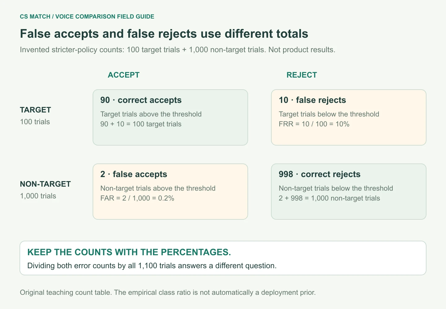
ROC and DET describe a threshold sweep
Lowering a higher-is-target threshold accepts more trials. It can reduce false rejects while increasing false accepts; raising it moves in the opposite direction. In the same invented example, a looser threshold rejects five targets and accepts eight non-targets, giving FRR five percent and FAR 0.8 percent. Neither pair of rates is universally better without a decision context.
A ROC curve relates false-positive rate to true-positive rate across thresholds; a DET representation uses false-positive and false-negative rates, often displayed on normal-deviate axes. Scikit-learn documents the underlying curve outputs. Specify axes and conventions rather than assume every error plot is directly comparable. Plotting a curve is an evaluation operation, not evidence that the deployed threshold was chosen independently.
Inspect the region that matters to the intended workload. A system can look attractive across much of a curve and still perform poorly at a required low false-alarm rate. Keep the numerical operating points and counts available. When scores tie, the finite set of attainable deterministic thresholds can leave gaps; do not hide interpolation or randomized-decision assumptions behind a smooth illustration.
| Invented policy | False accepts / non-target | False rejects / target |
|---|---|---|
| Stricter | 2 / 1000 = 0.2% | 10 / 100 = 10% |
| Looser | 8 / 1000 = 0.8% | 5 / 100 = 5% |
EER is a summary point, not every operating point
Equal error rate summarizes the point where false-alarm and miss rates meet, or an explicitly defined estimate of that crossing. A finite score list may not contain a threshold with exactly equal rates. Report the computation convention, especially with ties or few errors. BOSARIS discusses principled evaluation in these conditions rather than treating every software implementation as numerically identical.
EER is useful for comparing discrimination under a matched protocol, but it assigns a particular balance to two conditional errors. An application may care much more about one than the other. A lower EER does not guarantee a lower false-alarm rate at every selected threshold, nor does it supply a decision policy for a population with a different frequency of targets.
Do not turn a published EER into a universal accuracy percentage by subtracting it from one hundred. Dataset, trial design, source conditions and scoring configuration remain part of the result. Our checkpoint guide scopes its published benchmark separately. Current CS Match report percentages are not EER estimates and do not constitute an independently measured product accuracy claim.
Detection cost makes the decision assumptions explicit
A detection cost weights misses and false alarms using their costs and an assumed target prior. A common form multiplies miss rate by target prior and miss cost, then adds false-alarm rate weighted by non-target prior and false-alarm cost. State all parameters. A cost value without its prior and normalization does not identify one universal quality measure.
For teaching arithmetic, choose target prior 0.01 and unit costs for both errors. The stricter invented policy has cost 0.00298: 0.01 times 0.10 plus 0.99 times 0.002. The looser policy has cost 0.00842. The stricter choice is cheaper under these assumptions despite its larger miss rate. Changing the assumptions can change the preferred operating point.
Dividing by the better constant-decision cost, here 0.01, yields normalized costs 0.298 and 0.842. These are illustrative calculations, not NIST submission results or operational recommendations. The NIST plan specifies its own cost settings and aggregation. The assumed one-percent prior is a decision parameter in this example, not the empirical ratio of target trials in the invented list.
DCF = Cmiss × Ptarget × FRR + Cfa × (1 − Ptarget) × FAR.Default cost = min(Cmiss × Ptarget, Cfa × (1 − Ptarget)); normalized DCF = DCF / default cost.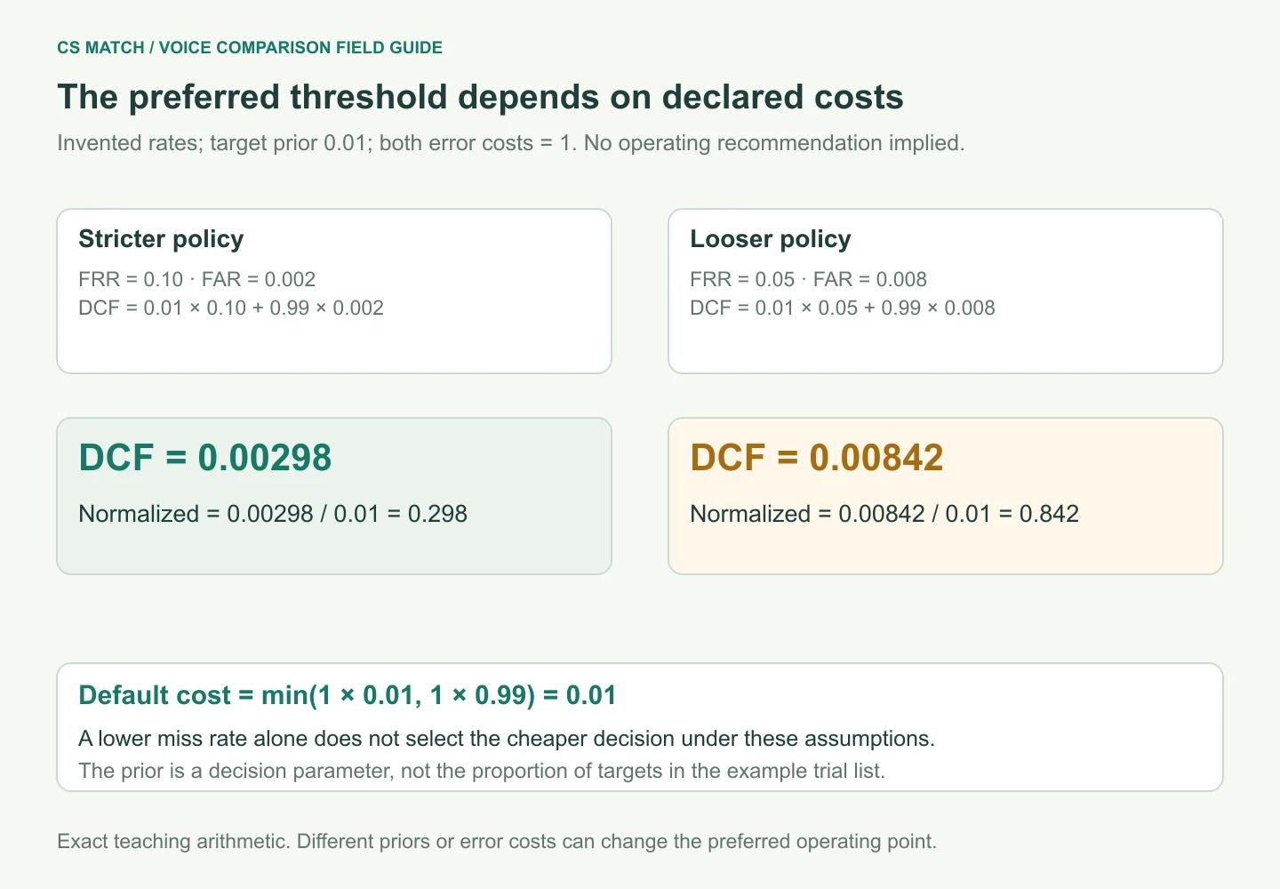
minDCF and actual cost answer different questions
Minimum detection cost searches the evaluated score list for the threshold giving the lowest cost under fixed parameters. It describes attainable threshold performance on those scores. It is not the cost guaranteed by a threshold chosen before seeing them. Searching the final test labels for the best cutoff is useful diagnostic analysis, but cannot be presented as an independently selected deployment policy.
Actual cost evaluates the declared operating rule, such as a fixed threshold chosen on development data or a decision threshold applied to calibrated likelihood ratios. Compare it with minimum cost under the same conditions. A gap can reveal problems with score interpretation or threshold transfer, while a poor minimum already indicates limited discrimination for that operating objective.
Keep normalized and unnormalized variants explicit, including the priors and error costs. A strictly increasing score remapping leaves the same threshold order available, so it need not improve minDCF even when it improves the meaning of an actual threshold. Evaluate the calibration or selection rule on independent trials rather than crediting it for a retrospectively optimized test-set cutoff.
Calibration connects evidence to a decision model
A likelihood ratio compares support for target and non-target hypotheses under a specified model. With an appropriate prior, posterior odds equal likelihood ratio times prior odds. The log-likelihood ratio adds to log prior odds. This distinguishes evidence from prevalence: identical acoustic evidence can lead to different posterior probabilities when the assumed population or decision setting changes.
Calibration can learn a mapping from raw scores using labelled development trials, for example through logistic-regression-based methods. It does not make incompatible embedding spaces compatible or remove dataset leakage. The calibration population and conditions matter. Research on condition-robust speaker backends explicitly studies failures when calibration conditions differ from evaluation conditions; one mapping should not be assumed universal.
Our application does not currently provide this calibrated likelihood-ratio or posterior-probability layer. Its categories should retain their technical meaning. If calibration is developed later, identify the training data, hypotheses, prior convention and evaluation metric, then assess held-out decisions. A probability-looking interface is not a substitute for that work, and calibration cannot create discrimination absent from the underlying scores.
Posterior odds = likelihood ratio × prior odds, under the stated hypotheses and model.Zero observed false accepts does not establish zero risk
An error estimate depends on the evidence supporting its denominator. Under an illustrative independent, identically distributed Bernoulli model, zero false accepts in one thousand non-target trials still gives a one-sided exact ninety-five-percent upper bound of approximately 0.299 percent. That is not a measured deployment rate; it shows why observing no errors does not prove the underlying probability is zero.
The calculation assumes independence and a common error probability. Audio trials often reuse speakers, sessions and references, so those assumptions may fail. A million pairs built from a small recording pool are not a million independent observations. Use an uncertainty method appropriate to the sampling structure and explain its limits rather than attach a simple binomial interval to every possible trial list.
SciPy documents exact and Wilson proportion intervals, while the VOiCES analysis demonstrates that speaker-aware resampling changes uncertainty assessment. Keep speakers and recordings visible in an evaluation record. Report counts, failed processing and condition coverage alongside intervals. Additional independent sources can improve evidence in ways that merely generating more combinations of the same windows cannot.
Teaching assumption: 0 errors in n=1000 independent Bernoulli trials.One-sided 95% exact upper bound = 1 − 0.05^(1/1000) ≈ 0.002991 = 0.2991%.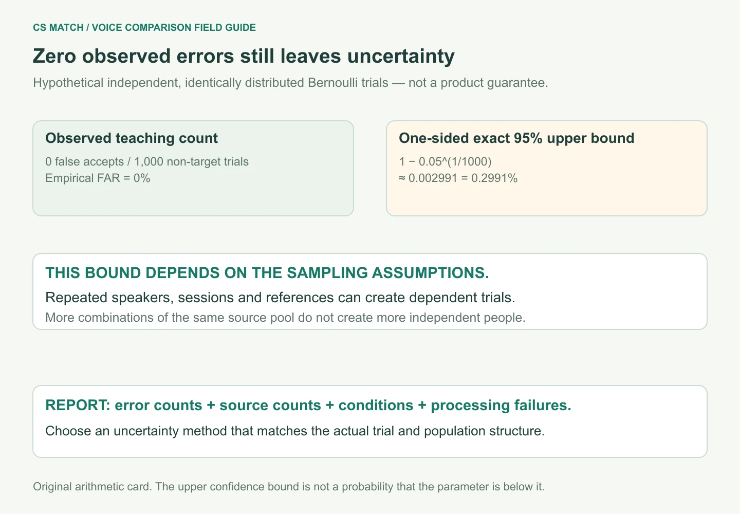
Include the population and failure policy in the metric
A benchmark should state which source channels, durations, languages and recording conditions it contains. Aggregate rates can hide a weak subgroup or a change in population mix. Report relevant condition-specific results with enough supporting evidence to interpret them. Avoid treating a missing condition as covered simply because the training corpus was broad or the model family is well known.
Define what happens when decoding, speech detection or embedding generation fails. A system evaluated only on successful preferred-engine jobs has a conditional scope. An operational policy may reject unusable material, request another sample or use another path; report that behaviour separately from errors on scored trials. Silently removing difficult failures can make a system appear better while reducing usable coverage.
The current worker has alternate embedding paths when the preferred model is unavailable. Those representations do not share an established learned space merely because a job completes. Retain engine provenance and avoid mixing their scores into a single claimed ECAPA benchmark. Distinguish process success, evidence sufficiency and recognition performance throughout the evaluation.
Evaluate the maximum-search workflow at its actual unit
Searching a long recording creates many candidate windows and then selects favourable evidence. The maximum score has a different distribution from a single preselected comparison. A longer search can offer more opportunities for an extreme non-target score even when the encoder is unchanged. Evaluate the recording-level decision that the workflow actually exposes instead of borrowing a clean-pair verification rate.
Neighbouring windows share speech, so they are not independent votes. Repeating a high score across overlapping windows can represent one passage rather than several confirmations. The median of a few selected best windows also depends on selection. Keep source times and evaluate full-recording positives and negatives when the task is finding a reference-like voice somewhere in a file.
Localization is another dimension. A recording-level target decision can be correct while its highlighted interval points to the wrong speaker or includes a long gap. Assess temporal evidence separately where it matters. Our merged ranges and estimated matched-speech coverage help navigation; they are not independent annotations of verified target speech or extra probabilities to multiply with the similarity score.
Read the current report with these metric boundaries
Best score is the strongest analysis-window comparison with the reference centroid. Top five median summarizes up to five highest scores. Matched duration describes retained merged spans, and matched-speech ratio estimates coverage using the implementation's speech information. These summaries answer different review questions. None is a measured FAR, FRR, EER or calibrated likelihood ratio.
To make a deployment claim, freeze the preparation, encoder, reference construction, search rule and threshold, then evaluate labelled independent trials. Publish the operating conditions, errors, uncertainty and processing coverage. The methods in this guide explain what such evidence would mean; they do not assert that those product-level measurements have already been collected.
For everyday review, listen to the reference and inspect several supporting passages, including contradictions and weak conditions. A technically strong resemblance can be useful for locating material without establishing identity or authenticity. Keeping metric definitions honest lets the report serve that purpose and gives future model improvements a clear, reproducible standard to meet.
Questions about this workflow
Is EER the percentage of wrong decisions at every threshold?
No. It summarizes a balanced-error crossing under a specified protocol. A chosen operating threshold has its own false-accept and false-reject rates.
Does minDCF tell us which threshold will work on new recordings?
No. It is a minimum over evaluated scores under declared costs and prior. Select a deployment rule on development data and assess its actual cost independently.
Does zero false accepts in a test prove the system is safe from false matches?
No. Sample size, independence and population coverage limit that conclusion. The zero-error example in this guide is teaching arithmetic, not a product guarantee.
Are current similarity percentages calibrated identity probabilities?
No. They describe technical resemblance or coverage under the current implementation. Calibration and independent product-level error measurements remain separate work.
Continue with the next useful step
Training and Evaluating Voice Comparison on Real Recordings
Build a reproducible speaker-comparison study: source labels, speaker and session splits, trial conditions, baseline checkpoints, adaptation, calibration, full-recording evaluation and uncertainty.
ECAPA-TDNN and VoxCeleb: Training, Checkpoints and Real-World Limits
Understand ECAPA-TDNN training, VoxCeleb trial protocols, pretrained checkpoints, augmentation, reproducibility and the limits of applying benchmark results to real voice comparison.
What Voice Similarity Scores Mean
Understand best score, top 5 median, matched speech, speaker summaries and technical similarity labels without treating them as identity probabilities.